2 Applied examples
In “Applying quantitative bias analysis in clinical and epidemiological studies using quantitative bias analysis” we present three applied examples of bias formulas, bounding methods, and probabilistic bias analysis. Code to generate results for these applied examples is presented below.
2.1 Bias formulas for selection bias
In a cohort study of pregnant women investigating the association between maternal lithium use, relative to non-use, and cardiac malformations in live-born infants, a covariate-adjusted risk ratio was estimated of 1.65 (95% CI, 1.02-2.68).(Patorno et al. 2017) Only live-born infants only were included in the study, and as such there was potential for selection bias if there were differences in termination probabilities of foetuses with cardiac malformations by exposure group.
Given that the outcome was rare, and therefore odds ratios and risk ratios are approximately equivalent, bias formulas using odds ratios were applied.(Greenland 1996)
\[ OR_{BiasAdjusted} = OR_{Observed}\frac{S_{01}S_{10}}{S_{00}S_{11}} \] Values for the bias parameters, selection probabilities by exposure and outcome status, were specified based on the literature. The selection probability of unexposed without cardiac malformations was assumed to be 0.8 (i.e. 20% probability of termination). The selection probability of unexposed with cardiac malformations was varied from 0.5 to 0.7. (30-50% probability of termination). Selection probabilities of exposed were defined by outcome status relative to unexposed (0% to -10% difference).
library(tidyverse)
library(ggplot2)

# Define observed odds ratio
observed_rr <- 1.65

# Define bias parameters
S00 <- 0.8
S01 <- c(0.5, 0.525, 0.55, 0.575, 0.6, 0.625, 0.65, 0.675, 0.7)
differences <- c(0, -0.05, -0.1)

# Define function to calculate bias-adjusted risk ratio
calc_bias_adj_or <- function(or, s01, s10, s00, s11) {
  bias_adj_or <- or * (s01*s10)/(s00*s11)
  return(bias_adj_or)
}

# Calculate bias-adjusted estimate for different values of bias parameters
results <- NULL
for (s01 in S01) {
  for (diff in differences) {
    bias_adj_rr <- calc_bias_adj_or(observed_rr, s01, S00 + diff, S00, s01 + diff)
    results_row <- tibble_row(bias_adj_rr=bias_adj_rr, s01=s01, diff=as.character(diff))
    results <- bind_rows(results, results_row)
  }
}

# Tidy label for difference in selection probabilities
results <- results %>%
  mutate(diff=factor(diff, levels=c("0", "-0.05", "-0.1"), labels=c("0", "-5%", "-10%")))

# Plot figure of bias-adjusted estimates
ggplot(data = results, aes(x=s01, y=bias_adj_rr, colour=diff)) +
  geom_line() +
  theme_minimal() +
  ylim(1.4, 2) +
  scale_x_reverse() +
  xlab("Selection probability of unexposed with cardiac malformations") +
  ylab("Bias-adjusted risk ratio") +
  guides(colour=guide_legend(title="Difference in selection\nprobability of exposed")) +
  theme(legend.title=element_text(size=10))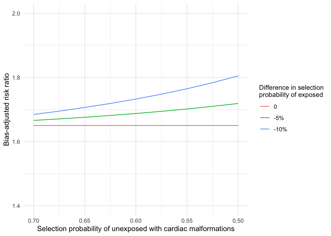
Figure 2.1: Bias-adjusted risk ratio for different assumed selection probabilities
The bias-adjusted risk ratios ranged from 1.65 to 1.80 (Figure 2.1), indicating robustness of the point estimate to selection bias under the given assumptions. We can likewise calculate bias-adjusted estimates for the lower bound of the confidence interval.
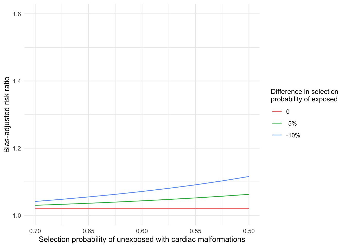
Figure 2.2: Bias-adjusted risk ratio for lower bound of 95% confidence interval for different assumed selection probabilities
2.2 E-values for unmeasured confounding
In a cohort study conducted in electronic health records investigating the association between proton pump inhibitors, relative to H2 receptor antagonists, and all-cause mortality, investigators found that individuals were at higher risk of death (covariate-adjusted hazard ratio [HR] 1.38, 95% CI 1.33-1.44).(Brown et al. 2021) However, it was considered that there may be unmeasured confounding due to differences in frailty between individuals prescribed proton pump inhibitors. The prevalence of the unmeasured confounder was not known in either exposure group, and therefore rather than use bias formulas, an E-value was calculated.(Ding and VanderWeele 2016)
Given the outcome was rare, the E-value method can be applied to the hazard ratio.
\[ \text{E-value} = RR_{Obs} + \sqrt{RR_{Obs}(RR_{Obs} -1)} \]
We can use the EValue package to calculate E-Values.
# load EValue package and ggplotify
library(EValue)

#Calculate E-values
evalues.HR(est=1.38, lo=1.33, hi=1.44, rare=TRUE) %>% knitr::kable()| point | lower | upper | |
|---|---|---|---|
| RR | 1.380000 | 1.330000 | 1.44 |
| E-values | 2.104155 | 1.992495 | NA |
And we can use bias_plot from the EValue package to display an E-value plot.
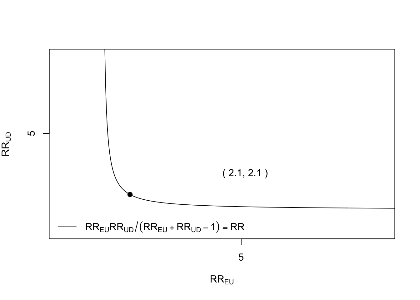
Figure 2.3: E-value plot for point estimate
The E-value for the point estimate was 2.10 and for the lower bound of the point estimate was 1.99. This represents the minimum strength of association that an unmeasured confounder would need to have with either exposure or outcome to reduce the hazard ratio to the null (i.e. 1). An unmeasured confounder with strength of association with exposure and outcome below the line in the plot could not possibly explain, on its own, the observed association.
Risk ratios between frailty and mortality >2 have been observed in the literature, and as such we could not rule out unmeasured confounding as a possible explanation for findings based on the E-value. However, as we did not specify prevalence of an unmeasured confounder, we cannot say whether such confounding was likely to account for the observed association. There may also have been additional unmeasured or partially measured confounders contributing to the observed association.
2.3 Probabilistic bias analysis for misclassification
In a cohort study of pregnant women conducted using insurance claims data, the observed covariate-adjusted risk ratio for the association between antidepressant use and congenital cardiac defects, was 1.02 (95% CI, 0.90-1.15).(Huybrechts et al. 2014) Some misclassification of the outcome, congenital cardiac malformation was anticipated. Therefore, probabilistic bias analysis was carried out.(Fox, Lash, and Greenland 2005) Code is not provided for this analysis, which was carrier out using SAS and participant record-level data (see sensmac macro for a SAS program to conduct this analysis).
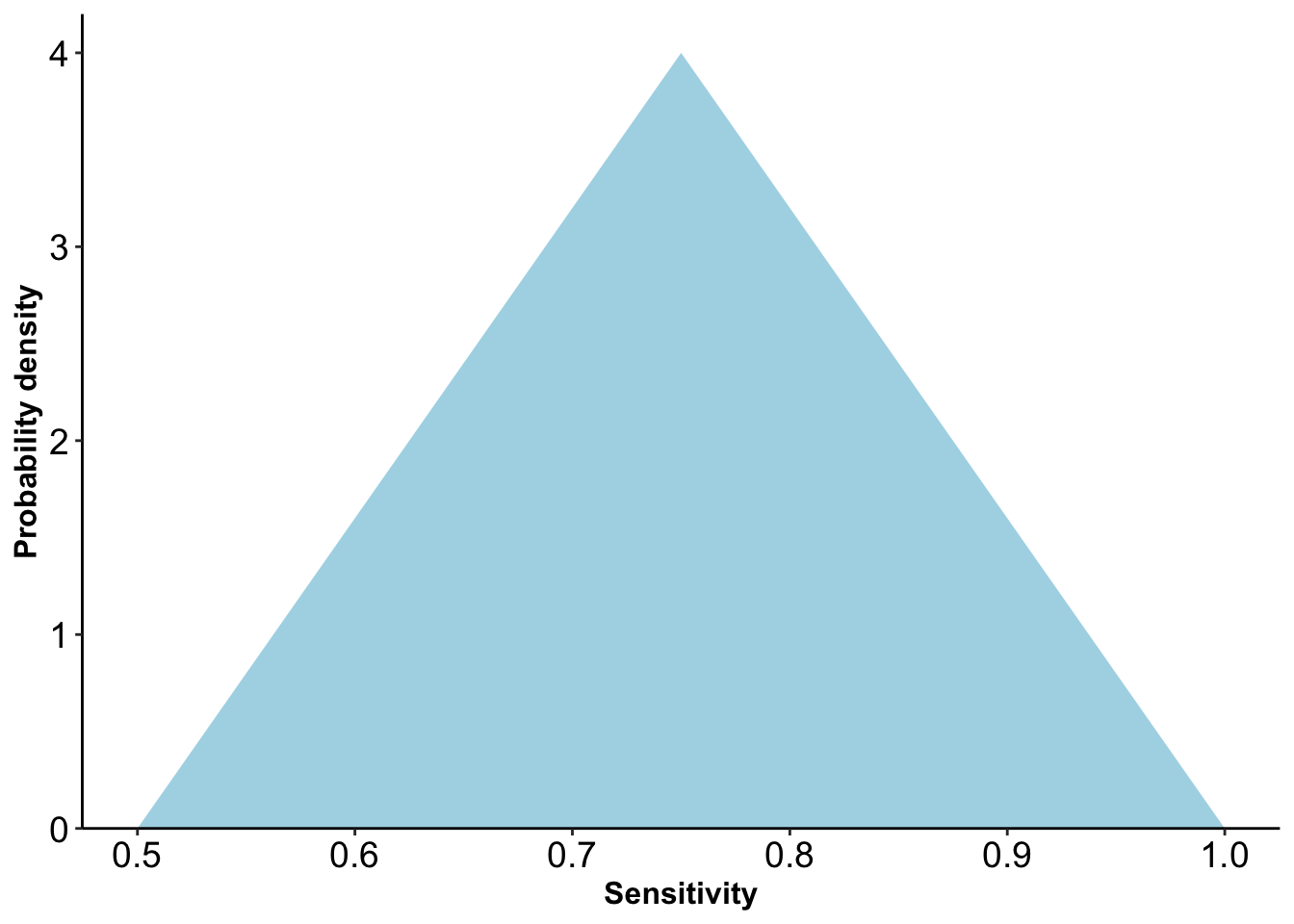
Figure 2.4: Triangular distribution for sensitivity
Positive predictive values estimated in a validation study were used to specify distributions of values for the bias parameters of sensitivity and specificity. Investigators chose triangular distributions for sensitivity and specificity (Figure 2.4).
Values were repeatedly sampled at random 1,000 times from these distributions and these sampled values were used to calculate a distribution of bias-adjusted estimates. The median bias-adjusted estimate was 1.06 with 95% simulation interval 0.92-1.22.