3 Additional example applications
We present here examples of quantitative bias analysis using simulated participant-level data for a cohort study with a binary treatment, binary outcome, and binary confounder.
3.1 Selection bias
In the simulated data we have a binary treatment \(A\), binary confounder \(X\), outcome \(Y\), and a binary indicator for selection into the study \(S\). A copy of the simulated data can be downloaded from GitHub.
## # A tibble: 5 × 4
##       x     a     y     s
##   <dbl> <dbl> <dbl> <dbl>
## 1     0     0     0     1
## 2     0     0     0     1
## 3     0     0     0     1
## 4     0     0     0     1
## 5     0     0     0     1
The data was generated such that the causal conditional odds ratio between treatment and outcome was 2. However, in a given sample the estimate may differ due to random error. If we observed a random sample from the target population we could unbiasedly estimate the odds ratio using logistic regression.
# fit logistic regression model
lgr_model <- glm(y ~ x + a, data=sim_data, family="binomial")

# tidy model outputs
or <- lgr_model %>%
  tidy(exponentiate=TRUE, conf.int=TRUE) %>%
  filter(term == "a") %>%
  select(estimate, conf.low, conf.high)

# output as table
or %>%
knitr::kable(caption = "Estimated odds ratio")| estimate | conf.low | conf.high |
|---|---|---|
| 2.040021 | 1.942229 | 2.142647 |
However, if we consider that selection into the study was dependent on exposure and outcome and that we only observed a selected subsample of the target population, then the estimated odds ratio is biased.
# restrict data to selected subsample
selected_data <- sim_data %>% filter(s == 1)

# fit logistic regression model
lgr_model_selected <- glm(y ~ x + a, data=selected_data, family="binomial")

# tidy model outputs
or_selected <- lgr_model_selected %>%
  tidy(exponentiate=TRUE, conf.int=TRUE) %>%
  filter(term == "a") %>%
  select(estimate, conf.low, conf.high)

# output as table
or_selected %>%
knitr::kable(caption = "Estimated odds ratio in selected sample")| estimate | conf.low | conf.high |
|---|---|---|
| 1.577843 | 1.494616 | 1.665406 |
3.1.1 Bias formulas
One option is to apply bias formulas for the odds ratio.
\[ OR_{BiasAdjusted} = OR_{Observed}\frac{S_{01}S_{10}}{S_{00}S_{11}} \] Given that the data was simulated we know the selection probabilities (\(S11=0.7\), \(S01=1\), \(S10=0.9\), \(S00=1\)) and can directly plug them in to estimate a bias-adjusted odds ratio. However, in practice we will not know these probabilities and will typically specify a range of values, or for probabilistic bias analysis a distribution of values.
# define bias parameters
S11 <- 0.7
S01 <- 1
S10 <- 0.9
S00 <- 1

# apply bias formula
bias_adjusted_or <- or_selected %>%
  mutate(across(c(estimate, conf.low, conf.high), ~ .x * (S01*S10)/(S11*S00)))

# output as table
bias_adjusted_or %>%
knitr::kable(caption = "Bias-adjusted odds ratio")| estimate | conf.low | conf.high |
|---|---|---|
| 2.028656 | 1.92165 | 2.141236 |
3.1.2 Weighting
Alternatively, we can weight the individual records by the inverse probability of selection and use bootstapping to calculate a confidence interval
library(boot)

# Add weights
selected_data_with_weights <- selected_data %>%
  mutate(prob_select = a*y*S11 + (1-a)*y*S01 + a*(1-y)*S10 + (1-a)*(1-y)*S00) %>%
  mutate(inverse_prob = 1/prob_select)

# define function to estimate weighted odds ratio (needed for bootstrap function)
calculate_weighted_or <- function(weighted_data, i) {
  weighted_lgr <- glm(y ~ x + a, family="binomial", data=weighted_data[i,], weights=inverse_prob)
  weighted_or <- coef(weighted_lgr)[["a"]] %>% exp()
  return(weighted_or)
}

# set seed of random number generator to ensure reproducibility
set.seed(747)

# bootstrap calculation of confidence intervals
bootstrap_estimates <- boot(selected_data_with_weights, calculate_weighted_or, R=1000)

# calculate bias-adjusted point estimate using entire selected subsample
point_estimate <- calculate_weighted_or(selected_data_with_weights, 1:nrow(selected_data_with_weights))

# calculate percentile bootstrap confidence interval
conf_int <- quantile(bootstrap_estimates$t, c(0.025, 0.975))

# output bias-adjusted estimate
tibble(estimate=point_estimate, conf.low=conf_int[[1]], conf.high=conf_int[[2]]) %>%
knitr::kable()| estimate | conf.low | conf.high |
|---|---|---|
| 2.031339 | 1.920888 | 2.135751 |
If we expect selection probabilities to differ within levels of covariates then we can specify different selection probabilities for different strata of covariates.
3.2 Misclassification
We will now consider some quantitative bias analysis methods for misclassification of a binary outcome. Similar approaches can be applied for misclassification of a binary exposure.
With differential misclassification of the outcome, the odds ratio is biased.
# load data
misclassified_data <- read_csv("data/simulated_data.csv") %>% select(x,a,m_y,s)

# fit logistic regression model with misclassified outcome
lgr_model_misclassified <- glm(m_y ~ x + a, data=misclassified_data, family="binomial")

# tidy model outputs
or_misclassified <- lgr_model_misclassified %>%
  tidy(exponentiate=TRUE, conf.int=TRUE) %>%
  filter(term == "a") %>%
  select(estimate, conf.low, conf.high)

# output as table
or_misclassified %>%
knitr::kable(caption = "Estimated odds ratio with misclassified outcome")| estimate | conf.low | conf.high |
|---|---|---|
| 1.737071 | 1.650733 | 1.827756 |
3.2.1 Bias formulas
Bias formulas for misclassification typically apply to 2x2 tables or 2x2 tables stratified by covariates and require us to specify the bias parameters of sensitivity and specificity. Given that the data was simulated, we know that sensitivity and specificity among the treated were 80% and 99%, and that sensitivity and specificity among the unexposed were 100%. In practice, we do not know these values, but can estimate them using validation studies and specify a range or, for probabilistic bias analysis, distribution of plausible values.
| A=1 | A=0 | |
|---|---|---|
| Y*=1 | a | b |
| Y*=0 | c | d |
| A=1 | A=0 | |
|---|---|---|
| Y=1 | A | B |
| Y=0 | C | D |
# specify bias parameters
sensitivity_a0 <-  1
sensitivity_a1 <- 0.8
specificity_a0 <- 1
specificity_a1 <- 0.99

# define function to correct 2x2 table
correct_two_by_two <- function(a, b, c, d, sensitivity_a0, sensitivity_a1, specificity_a0, specificity_a1) {
  A <- (a - (a + c)*(1-specificity_a1))/(sensitivity_a1 + specificity_a1 - 1)
  B <- (b - (b + d)*(1-specificity_a0))/(sensitivity_a0 + specificity_a0 - 1)
  C <- a + c - A
  D <- b + d - B
  return(c("A"=A,"B"=B,"C"=C,"D"=D))
}

# extract 2x2 table values
a_x0 <- misclassified_data %>% filter(m_y==1, a==1, x==0) %>% nrow()
b_x0 <- misclassified_data %>% filter(m_y==1, a==0, x==0) %>% nrow()
c_x0 <- misclassified_data %>% filter(m_y==0, a==1, x==0) %>% nrow()
d_x0 <- misclassified_data %>% filter(m_y==0, a==0, x==0) %>% nrow()
a_x1 <- misclassified_data %>% filter(m_y==1, a==1, x==1) %>% nrow()
b_x1 <- misclassified_data %>% filter(m_y==1, a==0, x==1) %>% nrow()
c_x1 <- misclassified_data %>% filter(m_y==0, a==1, x==1) %>% nrow()
d_x1 <- misclassified_data %>% filter(m_y==0, a==0, x==1) %>% nrow()

# correct 2x2 table
corr_two_by_two_x0 <- correct_two_by_two(a_x0, b_x0, c_x0, d_x0, sensitivity_a0, sensitivity_a1, specificity_a0, specificity_a1)
corr_two_by_two_x1 <- correct_two_by_two(a_x1, b_x1, c_x1, d_x1, sensitivity_a0, sensitivity_a1, specificity_a0, specificity_a1)

# extract corrected 2x2 table values
A_x0 <- corr_two_by_two_x0[[1]]
B_x0 <- corr_two_by_two_x0[[2]]
C_x0 <- corr_two_by_two_x0[[3]]
D_x0 <- corr_two_by_two_x0[[4]]
A_x1 <- corr_two_by_two_x1[[1]]
B_x1 <- corr_two_by_two_x1[[2]]
C_x1 <- corr_two_by_two_x1[[3]]
D_x1 <- corr_two_by_two_x1[[4]]

# calculate Mantel-Haenszel odds ratio
numerator <- A_x1*D_x1/(A_x1 + B_x1 + C_x1 + D_x1) + A_x0*D_x0/(A_x0 + B_x0 + C_x0 + D_x0)
denominator <- B_x1*C_x1/(A_x1 + B_x1 + C_x1 + D_x1) + B_x0*C_x0/(A_x0 + B_x0 + C_x0 + D_x0)

mh_estimate <- numerator/denominator
print(mh_estimate)
## [1] 2.003725We can use bootstrapping to calculate a confidence interval.
3.2.2 Record-level correction
For record-level correction we can as before calculate two by two tables, but as a second step use these to calculate predictive values which we can use to impute a corrected exposure.
# calculate predictive values
ppv_a1_x1 <- sensitivity_a1*A_x1/a_x1
ppv_a0_x1 <- sensitivity_a0*B_x1/b_x1
npv_a1_x1 <- specificity_a1*C_x1/c_x1
npv_a0_x1 <- specificity_a0*D_x1/d_x1
ppv_a1_x0 <- sensitivity_a1*A_x0/a_x0
ppv_a0_x0 <- sensitivity_a0*B_x0/b_x0
npv_a1_x0 <- specificity_a1*C_x0/c_x0
npv_a0_x0 <- specificity_a0*D_x0/d_x0

# impute outcome
misclassified_data <- misclassified_data %>% mutate(y = rbinom(100000, 1, ppv_a1_x1*a*m_y*x + ppv_a0_x1*(1-a)*m_y*x + (1-npv_a1_x1)*a*(1-m_y)*x + (1-npv_a0_x1)*(1-a)*(1-m_y)*x + ppv_a1_x0*a*m_y*(1-x) + ppv_a0_x0*(1-a)*m_y*(1-x) + (1-npv_a1_x0)*a*(1-m_y)*(1-x) + (1-npv_a0_x0)*(1-a)*(1-m_y)*(1-x)))

# fit a logistic regression model using imputed exposure
glm(y ~ a + x, family="binomial", data=misclassified_data) %>%
  tidy(exponentiate=TRUE) %>% filter(term == "a") %>% select(estimate)
## # A tibble: 1 × 1
## estimate
## <dbl>
## 1 2.013.2.3 Probabalistic bias analysis
Rather than specify a single or range of values for the bias parameters of sensitivity and specificity we can instead specify probability distributions for these parameters and apply probabilistic bias analysis. Here for simplicity we will assume the distributions are not correlated, but we could also generate correlated bias parameters.(Fox, MacLehose, and Lash 2022) We use bootstrapping to incorporate random error.
library(EnvStats)

# draw bias parameters from triangular distributions
sensitivity_a1 <- rtri(1000, min=0.75, mode=0.8, max=0.85)
specificity_a1 <- rtri(1000, min=0.985, mode=0.99, max=0.995)

# specify fixed bias parameters
sensitivity_a0 <-  1
specificity_a0 <- 1

# set seed for random number generator (for reproducibility)
set.seed(2041)

estimates <- NULL
for (i in 1:1000) {

  bootstrap_indices <- sample(1:nrow(misclassified_data), nrow(misclassified_data), replace=TRUE)

  # extract 2x2 table values
  a_x0 <- misclassified_data[bootstrap_indices,] %>% filter(m_y==1, a==1, x==0) %>% nrow()
  b_x0 <- misclassified_data[bootstrap_indices,] %>% filter(m_y==1, a==0, x==0) %>% nrow()
  c_x0 <- misclassified_data[bootstrap_indices,] %>% filter(m_y==0, a==1, x==0) %>% nrow()
  d_x0 <- misclassified_data[bootstrap_indices,] %>% filter(m_y==0, a==0, x==0) %>% nrow()
  a_x1 <- misclassified_data[bootstrap_indices,] %>% filter(m_y==1, a==1, x==1) %>% nrow()
  b_x1 <- misclassified_data[bootstrap_indices,] %>% filter(m_y==1, a==0, x==1) %>% nrow()
  c_x1 <- misclassified_data[bootstrap_indices,] %>% filter(m_y==0, a==1, x==1) %>% nrow()
  d_x1 <- misclassified_data[bootstrap_indices,] %>% filter(m_y==0, a==0, x==1) %>% nrow()

  # calculate corrected 2x2 table
  corr_two_by_two_x0 <- correct_two_by_two(a_x0, b_x0, c_x0, d_x0, sensitivity_a0, sensitivity_a1[i], specificity_a0, specificity_a1[i])
  corr_two_by_two_x1 <- correct_two_by_two(a_x1, b_x1, c_x1, d_x1, sensitivity_a0, sensitivity_a1[i], specificity_a0, specificity_a1[i])

  # extract corrected 2x2 table values
  A_x0 <- corr_two_by_two_x0[[1]]
  B_x0 <- corr_two_by_two_x0[[2]]
  C_x0 <- corr_two_by_two_x0[[3]]
  D_x0 <- corr_two_by_two_x0[[4]]
  A_x1 <- corr_two_by_two_x1[[1]]
  B_x1 <- corr_two_by_two_x1[[2]]
  C_x1 <- corr_two_by_two_x1[[3]]
  D_x1 <- corr_two_by_two_x1[[4]]

  # calculate Mantel-Haenszel odds ratio
  numerator <- A_x1*D_x1/(A_x1 + B_x1 + C_x1 + D_x1) + A_x0*D_x0/(A_x0 + B_x0 + C_x0 + D_x0)
  denominator <- B_x1*C_x1/(A_x1 + B_x1 + C_x1 + D_x1) + B_x0*C_x0/(A_x0 + B_x0 + C_x0 + D_x0)

  estimates <- bind_rows(estimates, tibble_row(bias_adj_or = numerator/denominator))
}

# calculate median and 95% simulation interval of bias-adjusted estimates
quantile(estimates$bias_adj_or, c(0.025, 0.5, 0.975))
## 2.5% 50% 97.5%
## 1.830828 2.009066 2.206712# plot distribution of bias-adjusted estimates
ggplot(data=estimates) +
geom_density(aes(x=bias_adj_or), fill="darkblue", alpha=0.5) +
xlab("Bias-adjusted odds ratio")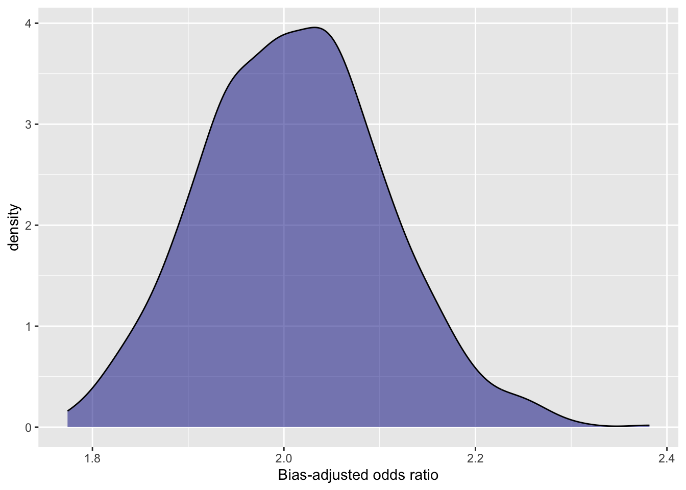
Figure 3.1: Distribution of bias-adjusted estimates
3.3 Unmeasured confounding
If the confounder, \(X\), had not been measured then we would not be able to adjust for it, and our estimates would be biased.
# restrict data to selected subsample
unmeasured_confounder_data <- sim_data %>% select(a,y)

# fit logistic regression model without confounder
lgr_model_confounded <- glm(y ~ a, family="binomial", data=unmeasured_confounder_data)

# tidy model outputs
or_confounded <- lgr_model_confounded %>%
  tidy(exponentiate=TRUE, conf.int=TRUE) %>%
  filter(term == "a") %>%
  select(estimate, conf.low, conf.high)

# output as table
or_confounded %>%
knitr::kable(caption = "Estimated odds ratio with unmeasured confounder")| estimate | conf.low | conf.high |
|---|---|---|
| 2.321895 | 2.213997 | 2.434989 |
3.3.1 Bias formula
Given that the outcome is rare we can apply a bias formula for the risk ratio.
\[ RR_{ZY}^{BiasAdj} = RR_{ZY}^{Obs}\frac{1 + P(U=1|Z=0)(RR_{UY|Z}-1)}{1 + P(U=1|Z=1)(RR_{UY|Z}-1)} \]
# define bias parameter
PU1 <- 0.33
PU0 <- 0.14
RR_UY <- 2

# define function to calculate bias-adjusted risk ratio
uconf_bias_adj_rr <- function(rr_zy, pu1, pu0, rr_uy) {
  bias_adj_rr <- rr_zy * (1 + pu0*(rr_uy - 1))/(1 + pu1*(rr_uy - 1))
  return(bias_adj_rr)
}

# calculate bias-adjusted odds ratios
or_confounded %>%
  mutate(across(c(estimate, conf.low, conf.high), ~ uconf_bias_adj_rr(.x, 0.33, 0.14, 2))) %>%
knitr::kable(caption = "Bias-adjusted odds ratio for unmeasured confounding")| estimate | conf.low | conf.high |
|---|---|---|
| 1.990196 | 1.897711 | 2.087134 |
3.4 Multiple biases
Finally, we consider a setting with both selection bias, misclassification, and unmeasured confounding.First, we correct for misclassification and selection to estimate the crude odds ratio, then we apply a bias formula to adjust for confounding bias.
multiple_bias_data <- read_csv("data/simulated_data.csv") %>% filter(s==1) %>% select(a,m_y)

# specify bias parameters
sensitivity_a0 <-  1
sensitivity_a1 <- 0.8
specificity_a0 <- 1
specificity_a1 <- 0.99

## record-level correction for misclassification
# extract 2x2 table values
a <- multiple_bias_data %>% filter(m_y==1, a==1) %>% nrow()
b <- multiple_bias_data %>% filter(m_y==1, a==0) %>% nrow()
c <- multiple_bias_data %>% filter(m_y==0, a==1) %>% nrow()
d <- multiple_bias_data %>% filter(m_y==0, a==0) %>% nrow()

# correct 2x2 table
corr_two_by_two <- correct_two_by_two(a, b, c, d, sensitivity_a0, sensitivity_a1, specificity_a0, specificity_a1)

# extract corrected 2x2 table values
A <- corr_two_by_two[[1]]
B <- corr_two_by_two[[2]]
C <- corr_two_by_two[[3]]
D <- corr_two_by_two[[4]]

# calculate predictive values
ppv_a1 <- sensitivity_a1*A/a
ppv_a0 <- sensitivity_a0*B/b
npv_a1 <- specificity_a1*C/c
npv_a0 <- specificity_a0*D/d

# impute outcome
multiple_bias_data <- multiple_bias_data %>% mutate(y = rbinom(nrow(multiple_bias_data), 1, ppv_a1*a*m_y + ppv_a0*(1-a)*m_y + (1-npv_a1)*a*(1-m_y) + (1-npv_a0)*(1-a)*(1-m_y)))

# calculate crude odds-ratio
multiple_bias_lgr <- glm(y ~ a,  family="binomial", data=multiple_bias_data)
or_adj_misc <- coef(multiple_bias_lgr)["a"] %>% exp()

# correct odds ratio for selection bias
or_adj_sel <- or_adj_misc * (S01*S10)/(S11*S00)

# apply bias formula for confounding
uconf_bias_adj_rr(or_adj_sel, 0.33, 0.14, 2)
## a
## 1.942437